Double kinematic wave option
Introduction
This annex describes the LISFLOOD double kinematic wave routine, and how it is used. Double kinematic wave routing is optional, and can be activated by adding the following line to the ‘lfoptions’ element the to LISFLOOD XML settings file:
<setoption name="SplitRouting" choice="1" />
Background
The flow routing is done by the kinematic wave approach. Therefore two equations have to be solved:
\[\frac{\partial Q}{\partial x} + \frac{\partial A}{\partial t} = q \rho {\kern 1pt} gA({S_0} - {S_f}) = 0\]where $A = \alpha \cdot {Q^{\beta} }$
The continuity equation momentum equation as expressed by Chow et al. 1988. With decreasing inflow the peaks of the resulting outflow will be later in time (see Figure below for a simple kinematic wave calculation). The wave propagation slows down because of more friction on the boundaries.
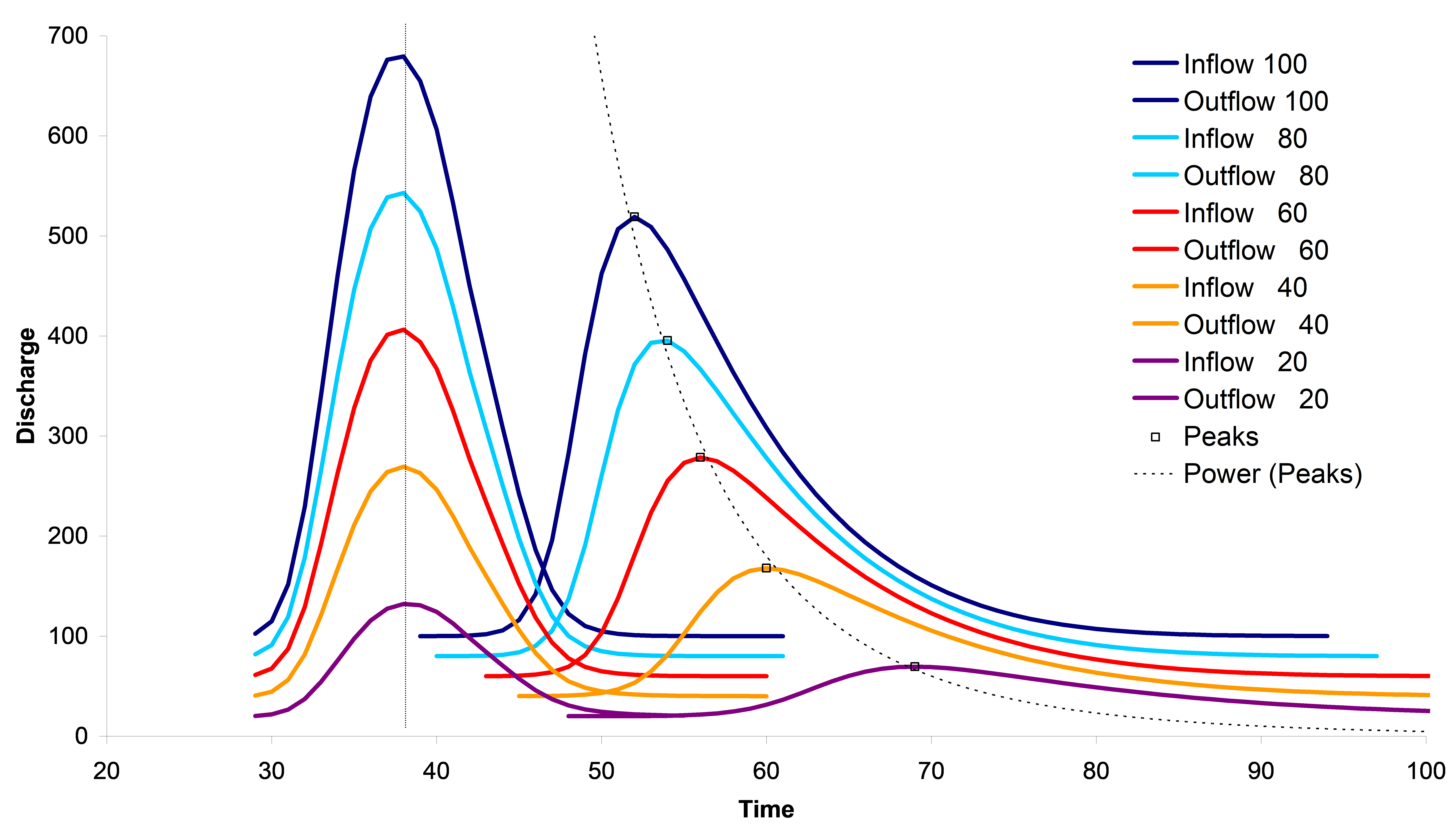 Figure: Simulated outflow for different amount of inflow wave propagation gets slower.
This is realistic if your channel looks like this:
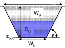
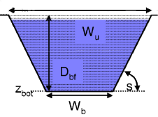 Figure: Schematic cross section of a channel with different water level.
But a natural channel looks more like this:
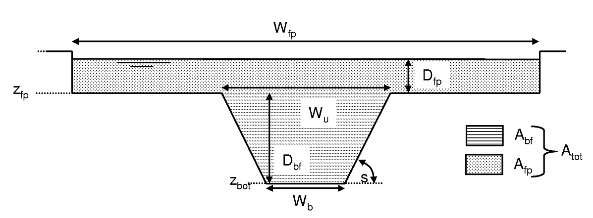 Figure: Schematic cross section of a natural channel.
Which means, opposite to the kinematic wave theory, the wave propagation gets slower as the discharge is increasing, because friction is going up on floodplains with shrubs, trees, bridges. Some of the water is even stored in the floodplains (e.g. retention areas, seepage retention). As a result of this, a single kinematic wave cannot cover these different characteristics of floods and floodplains.
Double kinematic wave approach
The double kinematic approach splits up the channel in two parts (see figure below):
1. bankful routing
2. over bankful routing
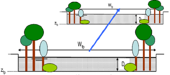
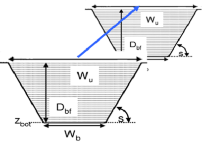 Figure: Channel is split in a bankful and over bankful routing
Similar methods are used since the 1970s e.g. as multiple linear or non linear storage cascade (Chow, 1988). The former forecasting model for the River Elbe (ELBA) used a three stages approach depending on discharge (Fröhlich, 1996).
The total water volume ($q_{ch} \cdot L{ch}$) entering the river system is computed as explained in the chapter channel routing is conveyed by the main channel, and, when the main channel flow capacity is exceeded, by the floodplain.
The total discharge $Q$ is partitioned between the main channel and the floodplain as follows:
$FlowRatio = ChannelVolume/(ChannelVolume+FloodplainVolume)$
$ChannelQ = FlowRatio \cdot Q$
$FlooplainQ = Q - ChannelQ$
Using double kinematic wave
No additional maps or tables are needed for initializing the double kinematic wave. A normal run (‘InitLisflood’=0) requires an additional map derived from the prerun (‘InitLisflood’=1). A ‘warm’ start (i.e. using initial values from a previous run) requires two additional maps with state variables for the second (over ‘bankful’ routing).
Table: Input/output double kinematic wave.
| Maps | Default name | Description | Units | Remarks |
|---|---|---|---|---|
| Average discharge | avgdis.map | Average discharge | $\frac{m^3}{s}$ | Produced by prerun |
| CrossSection2AreaInitValue | ch2cr000.xxx | channel crosssection for 2nd routing channel | $m^2$ | Produced by option ‘repStateMaps’ or ‘repEndMaps’ |
| PrevSideflowInitValue | chside00.xxx | sideflow into the channel | $mm$ |
Using the double kinematic wave approach option involves three steps:
1) In the ‘lfuser’ element (replace the file paths/names by the ones you want to use):
	<textvar>
	<textvar name="CalChanMan2" value="8.5">
	<comment>
	Channel Manning's n for second line of routing
	</comment>
	</textvar>
	<textvar name="QSplitMult" value="2.0">
	<comment>
	Multiplier applied to average Q to split into a second line of routing
	</comment>
	</textvar>
CalChanMan2 is a multiplier that is applied to the Manning’s roughness maps of the over bankful routing [-]
QSplitMult is a factor to the average discharge to determine the bankful discharge. The average discharge map is produced in the initial run (the initial run is already needed to get the groundwater storage). Standard is set to 2.0 (assuming over bankful discharge starts at 2.0·average discharge).
2) Activate the double kinematic wave option by adding the following line to the ‘lfoptions’ element:
<setoption name="SplitRouting" choice="1" />
3) Run LISFLOOD first with
<setoption name="InitLisflood" choice="1" />
and it will produce a map of average discharge $[\frac{m^3}{s}]$ in the initial folder. This map is used together with the QSplitMult factor to set the value for the second line of routing to start.
For a ‘warm start’ these initial values are needed
	<textvar name="CrossSection2AreaInitValue" value="-9999">
	<comment>
	initial channel crosssection for 2nd routing channel
	-9999: use 0
	</comment>
	</textvar>
	<textvar name="PrevSideflowInitValue" value="-9999">
	<comment>
	initial sideflow for 2nd routing channel
	-9999: use 0
	</comment>
	</textvar>
CrossSection2AreaInitValue is the initial cross-sectional area $[m^2]$ of the water in the river channels (a substitute for initial discharge, which is directly dependent on this). A value of -9999 sets the initial amount of water in the channel to 0.
PrevSideflowInitValue is the initial inflow from each pixel to the channel [mm]. A value of -9999 sets the initial amount of sideflow to the channel to 0.