Polder option
Introduction
This page describes the LISFLOOD polder routine, and how it is used. The simulation of polders is optional, and it can be activated by adding the following line to the ‘lfoptions’ element of the settings file:
<setoption name="simulatePolders" choice="1" />
The current implementation of the polder routine may result in numerical instabilities for kinematic wave pixels, so for the moment it is recommended to define polders only on channels where the dynamic wave is used.
Description of the polder routine
Polders are simulated as points in the channel network. The polder routine is adapted from Förster et. al (2004), and based on the weir equation of Poleni (Bollrich & Preißler, 1992). The flow rates from the channel to the polder area and vice versa are calculated by balancing out the water levels in the channel and in the polder, as shown in the following Figure:
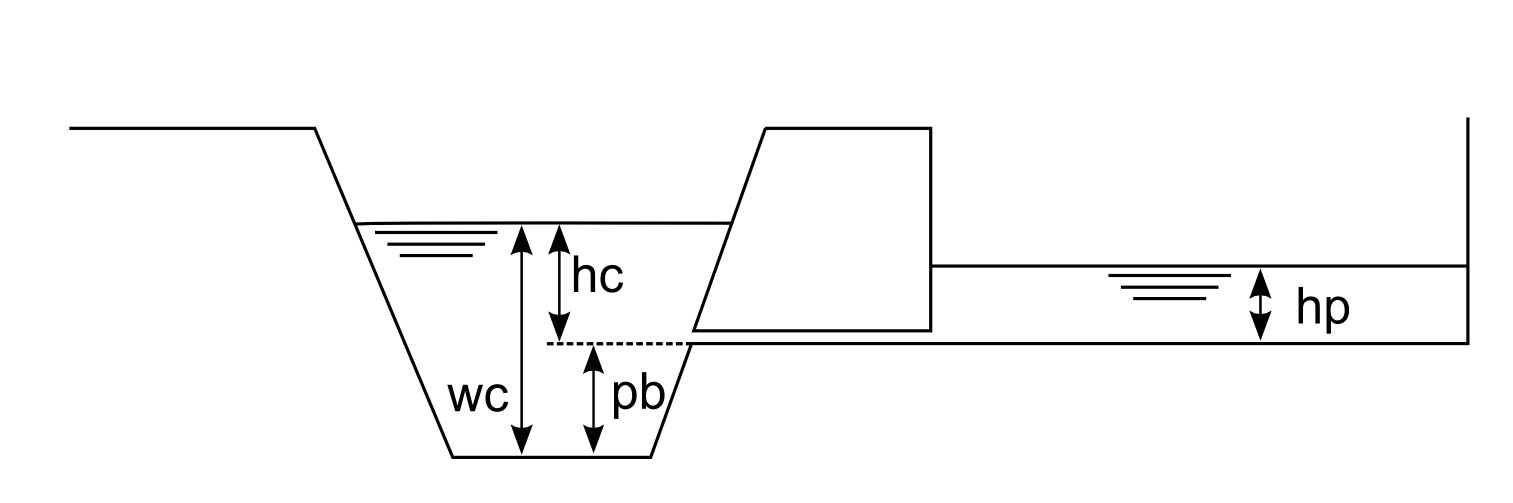 Figure: Schematic overview of the simulation of polders. $p_b$ is the polder bottom level (above the channel bottom); $w_c$ is the water level in the channel; $h_c$ and $h_p$ are the water levels above the polder in- / outflow, respectively
From the Figure, it is easy to see that there can be three situations:
-
$h_c > h_p$: water flows out of the channel, into the polder. The flow rate, $q_{c,p}$ [$\frac{m^3}{s}$], is calculated using:
\[\begin{array}{|ll} q_{c,p} = \mu \cdot c \cdot b \cdot \sqrt{2g} \cdot h_c^{3/2} \\ c = \sqrt{1 - [\frac{h_p}{h_c}]^{16}}\end{array}\]where
$b$ is the outflow width $[m]$,
$g$ is the acceleration due to gravity ($9.81\ \frac{m}{s^2}$),
$\mu$ is a weir constant which has a value of 0.49,
$c$ is the weir factor. -
$h_c < h_p$: water flows out of the polder back into the channel. The flow rate, $q_{p,c}$ [$\frac{m^3}{s}$] is now calculated using:
\[\begin{array}{|ll} q_{p,c} = \mu \cdot c \cdot b\sqrt{2g} \cdot h_p^{3/2} \\ c = \sqrt {1 - [\frac{h_c}{h_p}]^{16}}\end{array}\] -
$h_c = h_p$: no water flowing into either direction (note here that the minimum value of $h_c$ is zero). In this case both $q_{c,p}$ and $q_{p,c}$ are zero.
Regulated and unregulated polders
The above equations are valid for unregulated polders. The functioning of regulated polders is simulated according to the schematic shown in the following Figure.
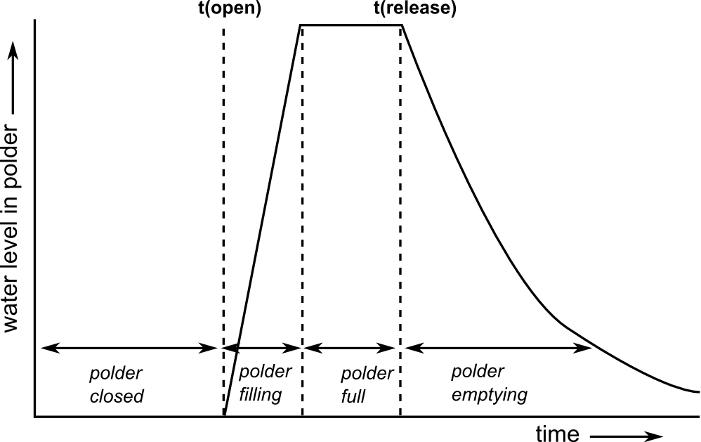 Figure: Simulation of a regulated polder. Polder is closed (inactive) until user-defined opening time, after which it fills up to its capacity (the flow rate is $q_{c,p}$ and it is computed using the above defined equation).
Water stays in polder until user-defined release time, after which water is released back to the channel (flow rate is now $q_{p,c}$ and it is computed using the above defined equation).
Figure: Simulation of a regulated polder. Polder is closed (inactive) until user-defined opening time, after which it fills up to its capacity (the flow rate is $q_{c,p}$ and it is computed using the above defined equation).
Water stays in polder until user-defined release time, after which water is released back to the channel (flow rate is now $q_{p,c}$ and it is computed using the above defined equation).
Regulated polders are opened at a user-defined time (typically during the rising limb of a flood peak). The polder closes automatically once it is full. Subsequently, the polder is opened again to release the stored water back into the channel, which also occurs at a user-defined time. The opening- and release times for each polder are defined in two lookup tables. In order to simulate the polders in unregulated mode these times should both be set to a bogus value of -9999. Only if both opening- and release time are set to some other value, LISFLOOD will simulate a polder in regulated mode. Since LISFLOOD only supports one single regulated open-close-release cycle per simulation, you should use regulated mode only for single flood events. For continuous simulations (e.g. long-tem waterbalance runs), it is recommended to use the unregulated mode.
Preparation of the input data
The locations of the polders are defined on a (nominal) map called ‘polders.map’. Any polders that are not on a channel pixel are ignored by LISFLOOD, so you may want to check the polder locations before running the model (you can do this by displaying the polder map on top of the channel map). The current implementation of the polder routine may result in numerical instabilities for kinematic wave pixels, so for the moment it is recommended to define polders only on channels where the dynamic wave is used. The properties of each polder are described using a number of tables. All the required input data are listed below:
Table: Input requirements polder routine.
| Maps | Defaultname | Description | Units | Remarks |
|---|---|---|---|---|
| PolderSites | polders.map | polder locations | - | nominal |
| Tables | Defaultname | Description | Units | Remarks |
| TabPolderArea | poldarea.txt | polder area | $m^2$ | |
| TabPolderOFWidth | poldofw.txt | polder in- and outflow width | $m$ | |
| TabPolderTotalCapacity | poldcap.txt | polder storage capacity | $m^3$ | |
| TabPolderBottomLevel | poldblevel.txt | Bottom level of polder, measured from channel bottom level (see also Figure above) | $m$ | |
| TabPolderOpeningTime | poldtopen.txt | Time at which polder is opened | $time step$ | |
| TabPolderReleaseTime | poldtrelease.txt | Time at which water stored in polder is released again | $time step$ |
Note that the polder opening- and release times are both defined a time step numbers (not days or hours!!). For unregulated polders, set both parameters to a bogus value of -9999, i.e.:
10 -9999
15 -9999
16 -9999
17 -9999
Preparation of settings file
All in- and output files need to be defined in the settings file. If you are using a default LISFLOOD settings template, all file definitions are already defined in the ‘lfbinding’ element. Just make sure that the map with the polder locations is in the “maps” directory, and all tables in the ‘tables” directory. If this is the case, you only have to specify the initial reservoir water level in the polders. PolderInitialLevelValue is defined in the ‘lfuser’ element of the settings file, and it can be either a map or a value. The value of the weir constant μ is also defined here, although you should not change its default value. So we add this to the ‘lfuser’ element (if it is not there already):
	<group>
	<comment>
	**************************************************************
	POLDER OPTION
	**************************************************************
	</comment>
	<textvar name="mu" value="0.49">
	<comment>
	Weir constant [-] (Do not change!)
	</comment>
	</textvar>
	<textvar name="PolderInitialLevelValue" value="0">
	<comment>
	Initial water level in polder [m]
	</comment>
	</textvar>
	</group>
To switch on the polder routine, add the following line to the ‘lfoptions’ element:
<setoption name="simulatePolders" choice="1" />
Now you are ready to run the model. If you want to compare the model results both with and without the inclusion of polders, you can switch off the simulation of polders either by:
- Removing the ‘simulatePolders’ statement from the ‘lfoptions element, or
- changing it into <setoption name="simulatePolders" choice="0" />
Both have exactly the same effect. You don’t need to change anything in either ‘lfuser’ or ‘lfbinding’; all file definitions here are simply ignored during the execution of the model.
Polder output files
The polder routine produces 2 additional time series and one map (or stack of maps, depending on the value of LISFLOOD variable ReportSteps), as listed in the following table:
Table: Output of polder routine.
| Maps / Time series | Default name | Description | Units |
|---|---|---|---|
| PolderLevelState | hpolxxxx.xxx | water level in polder at last time step | $m$ |
| PolderLevelTS | hPolder.tss | water level in polder (at polder locations) | $m$ |
| PolderFluxTS | qPolder.tss | Flux into and out of polder (positive for flow from channel to polder, negative for flow from polder to channel) | $\frac{m^3}{s}$ |
Note that you can use the map with the polder level at the last time step to define the initial conditions of a succeeding simulation, e.g.:
<textvar name="PolderInitialLevelValue" value="/mycatchment/hpol0000.730">
Limitations
For the moment, polders can be simulated on channel pixels where dynamic wave routing is used. For channels where the kinematic wave is used, the routine will not work and may lead to numerical instabilities or even model crashes. This limitation may be resolved in future model versions.