Preferential bypass flow

For the simulation of preferential bypass flow –i.e. flow that bypasses the soil matrix and drains directly to the groundwater- no generally accepted equations exist. Because ignoring preferential flow completely will lead to unrealistic model behavior during extreme rainfall conditions, a very simple approach is used in LISFLOOD. During each time step, a fraction of the water that is available for infiltration ($W_{av}$) is added to the groundwater directly (i.e. without first entering the soil matrix). It is assumed that this fraction is a power function of the relative saturation of the superficial and upper soil layers. This results in an equation that is somewhat similar to the excess soil water equation used in the HBV model (e.g. Lindström et al., 1997):

\[D_{pref,gw} =W_{av} \cdot (\frac{w_1}{w_{s1}})^{c_{pref}}\]

where $D_{pref,gw}$ is the amount of preferential flow per time step $[mm]$, $W_{av}$ is the amount of water that is available for infiltration, and $c_{pref}$ is an empirical shape parameter. The equation results in a preferential flow component that becomes increasingly important as the soil gets wetter. It is here noted that the preferential flow is only simulated in the permeable fraction of each pixel, defined as: $( 1 - f_{dr} )$, where $f_{dr}$ is the ‘direct runoff fraction’ [-]. The ‘direct runoff fraction’ is the fraction of a pixel occupied by urban areas and open water bodies.

The Figure below shows with $c_{pref} = 0$ (red line) all the available water for infiltration is converted into preferential flow and it bypasses the soil. $c_{pref} = 1$ (black line) gives a linear relation e.g. at 60% soil saturation 60% of the available water is bypassing the soil matrix. With increasing $c_{pref}$ the percentage of preferential flow is decreasing.

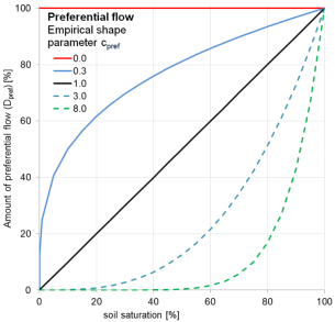
Figure: Soil moisture and preferential flow relation.