Snow Melt

In order to achieve an accurate represenation of the catchment hydrological processes, it is important to partition the measured precipitation into rain and snow. This distinction is controlled by the average temperature ($T_{avg}$). If $T_{avg}$ is below a threshold $TempSnow$, all the measured precipitation is assumed to be snow; the value $TempSnow = 1^\circ C$ is recommended. A snow correction factor $SnowFactor$ is then applied to correct for undercatch of snow precipitation. Undercatch in this context refers to the mismeasurement of snowfall by a precipitation measuement instrument. For instance, when using traditional rain gauges,wind gusts can blow some of the snow away from the gauge, or, vice-versa, accumulate snow within the gauge. The computation is summarised as follows:

• If $T_{avg} \lt TempSnow$: $Snow = SnowFactor \cdot Precipitation$
• Else If $T_{avg} \ge TempSnow$: $Rain = Precipitation$

Differently from rain, snow accumulates on the soil surface until it melts. The rate of snowmelt is estimated using a simple degree-day factor method. Degree-day factor type snow melt models usually take the following form (e.g. see WMO, 1986):

\[M = {C_m}({T_{avg}} - {TempMelt}) \cdot \Delta t\]

where

• M is the snowmelt per time step $[mm]$,
• $C_m$ is a degree-day factor $[\frac{mm} {°C \ day}]$,
• $T_{avg}$ is the average daily temperature $[°C]$,
• $TempMelt$ is the average temperature at which snow melts $[°C]$, and
• $\Delta t$ is the time interval $[days]$. $\Delta t$ can be <1 day.

Speers et al. (1979) developed an extension of this equation which accounts for accelerated snowmelt that takes place when it is raining (cited in Young, 1985). The equation is supposed to apply when rainfall is greater than 30 mm in 24 hours. Moreover, although the equation is reported to work sufficiently well in forested areas, it is not valid in areas that are above the tree line, where radiation is the main energy source for snowmelt). LISFLOOD uses a variation on the equation of Speers et al. The modified equation simply assumes that for each mm of rainfall, the rate of snowmelt increases with 1% (compared to a ‘dry’ situation). This yields the following equation:

\[M = ({C_m} + C_{Seasonal})(1 + 0.01 \cdot R\Delta t)(T_{avg} - T_m) \cdot \Delta t\]

where

• M is the snowmelt per time step $[mm]$,
• $C_m$ is a degree-day factor $[\frac{mm} {^\circ C \cdot day}]$,
• $C_{Seasonal}$ is a degree-day factor introduced to account for seasonal effects $[\frac{mm} {^\circ C \cdot day}]$,
• R is rainfall (not snow!) intensity $[\frac {mm}{day}]$,
• $T_{avg}$ is the average daily temperature $[°C]$,
• $TempMelt$ is the average temperature at which snow melts $[°C]$, and
• $\Delta t$ is the time interval $[days]$. $\Delta t$ can be $<1 day$.

$TempMelt$ can be defined by the user, the value $TempMelt = 1^\circ C$ is recommended. It must be stressed that the value of $C_m$ can vary greatly both in space and time (e.g. see Martinec et al., 1998). Therefore, in practice this parameter is used as calibration parameter. A low value of $C_m$ indicates slow snow melt. $C_{Seasonal}$ is a seasonal variable melt factor which is also used in several other models (e.g. Anderson 2006, Viviroli et al., 2009). There are mainly two reasons to use a seasonally variable melt factor:

• The solar radiation has an effect on the energy balance and varies with the time of the year.

• The albedo of the snow has a seasonal variation, because fresh snow is more common in the mid winter and aged snow in the late winter/spring. This produce an even greater seasonal variation in the amount of net solar radiation

The following Figure shows an example where a mean value $C_m = 3.0 \frac{mm}{^\circ C \cdot day}$ is modulated using $C_{Seasonal}$. The value of $C_m$ is reduced by $0.5$ at $21^{st}$ December and a $0.5$ is added on the $21^{st}$ June. In between a sinus function is applied. It is noted that this example refers to the Northern emisphere (LISFLOOD clearly accounts for the different seasons in the Northern and Southern Hemisphere).

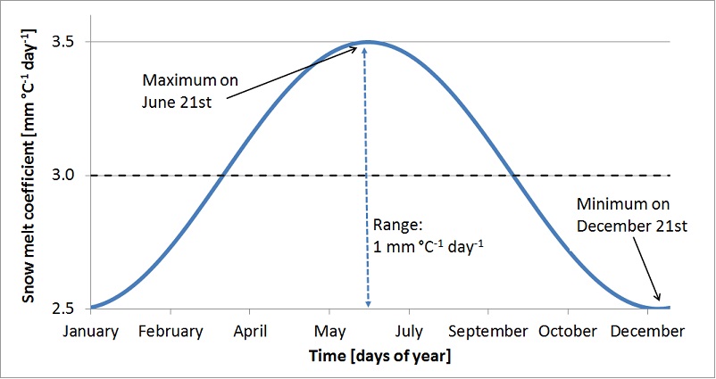
Figure: Sinus shaped snow melt coefficient ($C_m$) as a function of days of year.

At high altitudes, where the temperature never exceeds $1^\circ C$, the model accumulates snow without any reduction because of melting loss. In these altitudes runoff from glacier melt is an important part. The snow will accumulate and converted into firn. Then firn is converted to ice and transported to the lower regions. This can take decades or even hundred years. In the ablation area the ice is melted. In LISFLOOD this process is emulated by melting the snow in higher altitudes on an annual basis over summer. A sinus function is used to start ice melting ($Im$) in summer using the average temperature:

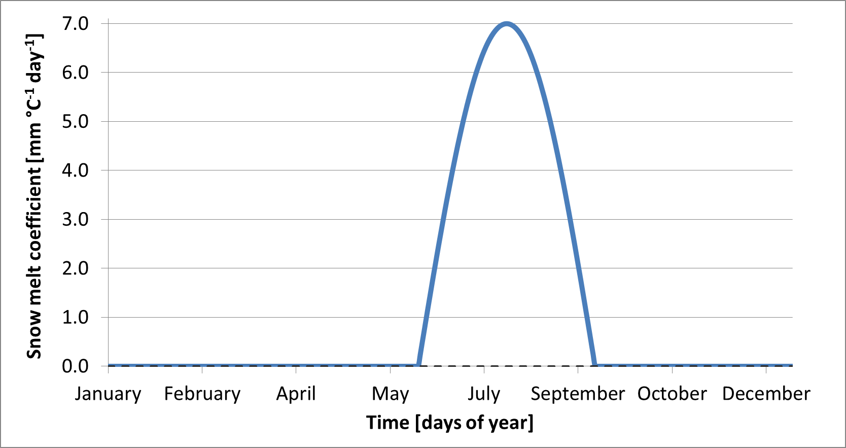
Figure: Sinus shaped ice melt coefficient as a function of days of year. As an example, this graph refers to the Northern Hemisphere

Clearly, at each time step, the total amount of snowmelt $M$ and ice melt $Im$ can never exceed the actual snow cover that is present on the surface.

For large pixel sizes, there may be considerable sub-pixel heterogeneity in snow accumulation and melt, which is a particular problem if there are large elevation differences within a pixel. Because of this, snow melt and accumulation are modelled separately for 3 separate elevation zones, which are defined at the sub-pixel level. This is shown in Figure below:

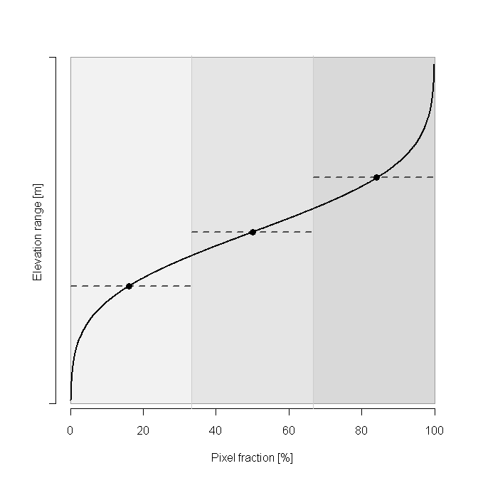
Figure: Definition of sub-pixel elevation zones for snow accumulation and melt modelling. Snowmelt and accumulation calculations in each zone are based on elevation (and derived temperature) in centroid of each zone.

The division in elevation zones is based on a normal distribution, which was found to adequately fit the real distribution of the elevation of e.g. 100m SRTM DEM pixels within a 5x5km grid cell. Three elevation zones A, B, and C are defined with each zone occupying one third of the pixel surface. Assuming further that $T_{avg}$ is valid for the average pixel elevation, average temperature is extrapolated to the centroids of the lower (A) and upper (C) elevation zones, using a fixed temperature lapse rate, L, of 0.0065 °C per meter elevation difference. Snow, snowmelt and snow accumulation are subsequently modelled separately for each elevation zone, assuming that temperature can be approximated by the temperature at the centroid of each respective zone.

At each time step, and in each elevation zone, the snow cover (expressed as mm equivalent water depth) is given by the sum of the precipitation as snow minus the snow melt and the ice melt:

\[SnowCover = Snow - M - Im\]

🔝