2. Potential reference evapo(trans)piration
LISVAP offers two internal possibilities to compute reference evapotranspiration:
- Penman-Monteith
- Hargreaves
1) Penman-Monteith equation
Reference values for potential evapotranspiration and evaporation are estimated using the Penman-Monteith equation (Supit et al., 1994, Supit & Van Der Goot, 2003).Specifically, the potential reference evapotranspiration rate [mm/day] for the reference vegetation canopy is computed as follows:
\[ET0 = \frac{\Delta R_{na} + \gamma EA}{\Delta + \gamma}\]where
$ET0$: is the potential evapotranspiration rate from reference vegetation canopy (closed vegetation canopy) $[\frac{mm}{day}]$
$R_{na}$: is the net absorbed radiation for the reference vegetation canopy $[\frac{mm}{day}]$
$EA$: is the evaporative demand of the reference vegetation canopy $[\frac{mm}{day}]$
$\Delta$: is the slope of the saturation vapour pressure curve $[\frac{mbar}{^\circ C}]$
$\gamma$: is the psychrometric constant $[\frac{mbar}{^\circ C}]$
The same equation is also used to estimate the potential evaporation from a water surface and the evaporation from a (wet) bare soil surface. This purpose is achieved by using different values for the net absorbed radiation term and for the evaporative demand.
The potential evaporation rate from a bare soil surface [mm/day] is then estimated by: s \(ES0 = \frac{\Delta R_{na,s} + \gamma EA_s}{\Delta + \gamma}\)
Finally, the potential evaporation rate from water surface [mm/day] is computed as follows:
\[EW0 = \frac{\Delta R_{na,w} + \gamma EA_w}{\Delta + \gamma}\]where $R_{na,s}$ and $R_{na,w}$ are the net absorbed radiation of bare soil surface and the net absorbed radiation of water surface, respectively ($[\frac{mm}{day}]$); $EA_s$ and $EA_w$ are the evaporative demand of bare soil surface and the evaporative demand of water surface, respectively ($[\frac{mm}{day}]$).
The procedure to calculate potential evapo(transpi)ration is summarised in the following Figure.
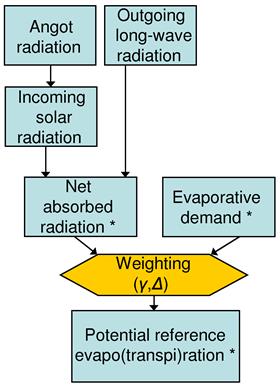
Figure: Overview of procedure to calculate potential reference evapo(transpi)ration. Terms with an asterisk (*) are calculated separately for a reference vegetation canopy, a bare soil surface and an open water surface, respectively.
The table below lists the properties of the reference surfaces that are used in the computation of $ET0$, $ES0$ and $EW0$, respectively.
| α (surface albedo) | fc (empirical constant in evaporative demand equation) | |
|---|---|---|
| $ET0$ | 0.23 | 1 |
| $ES0$ | 0.15 | 0.75 |
| $EW0$ | 0.05 | 0.5 |
Calculating net absorbed radiation
Calculating the net absorbed radiation term involves the following two steps:
- Calculate the Angot radiation (daily extra-terrestrial radiation)
- Calculate the net absorbed radiation
Some data sets (e.g. ERA5) provide pre-calculated values for both incoming solar radiation and net long-wave radiation. When both the datasets are available, LISVAP offers the possibility to use these values directly. Conversely, LISVAP applies the following protocol to compute the Angot radiaton.
Step 1: Angot radiation (daily extra-terrestrial radiation)
The daily extra-terrestrial radiation is the product of the solar constant at the top of the atmosphere and the integral of the solar height over the day:
\[R_{a,d} = S_{c, d} \int sin \ \beta \ dt_h\]where
$R_{a,d}$: Daily extra-terrestrial radiation $[{\frac{J}{m^2 \ day}}]$
$S_{c,d}$: Solar constant at the top of the atmosphere $[{\frac{J}{m^2 \ s}}]$
$\int sin \ \beta \ dt_h$: Integral of the solar height over the day $[s]$
The solar constant on a given day is calculated as:
where
$S_c$: Average solar radiation at the top of the atmosphere $[{\frac{J}{m^2 \ s}}]$ (= 1370 ${\frac{J}{m^2 \ s}}$)
$S_{c,d}$: Solar constant at the top of the atmosphere $[{\frac{J}{m^2 \ s}}]$
$t_d$: Calendar day number (1st of January is 1, etcetera) $[-]$
The calendar day number is always a number between 1 and 365.25 (taking into account leap years, a year has on average 365.25 days).
The integral of the solar height equals:
where
$L_d$: Astronomical day length $[h]$
$\delta$: Solar declination $[^\circ]$
$\lambda$: Latitude $[^\circ]$
with:
\[B_{ld} = \frac{-sin (\frac{PD}{\pi})+sin \ \delta \cdot sin \ \lambda}{cos \ \delta \cdot \ cos \ \lambda}\]where PD is a correction constant (-2.65).
The solar declination is a simple function of the calendar day number (td):
The day length is given by:
Step 2: Net absorbed radiation
The net absorbed radiation is calculated for three reference surfaces:
- Reference vegetation canopy
- Bare soil surface
- Open water surface
The following equation is used to calculate the net long-wave radiation[1] (Maidment, 1993):
\[R_{nl}= f \epsilon \sigma (T_{av}+273)^4\]where
$R_{nl}$: Net long-wave radiation $[{\frac{J}{m^2 \ day}}]$
$\sigma$: Stefan Boltzmann constant: $4.903 \cdot 10^{-3}[{\frac{J}{m^2 \ K^4 \ day}}]$
$f$: Adjustment factor for cloud cover
$\epsilon$: Net emissivity between the atmosphere and the ground
The net emissivity is calculated as:
\[\epsilon = 0.56 - 0.079 \sqrt{e_a}\]where
$e_a$: Actual vapour pressure $[mbar]$
The actual vapour pressure ea can be provided as input data or computed as a function of the surface pressure and of the near-surface specific humidity:
\[e_a = \frac{( P_{surf} \cdot Q_{air} )}{62.2}\]where
$P_{surf}$: instantaneous sea level pressure $[pa]$
$Q_{air}$: 2 m instantaneous specific humidity [-]
Alternatively, when the weather stations provide the dew point temperature $T_{dew}$, the actual vapour pressure can be computed using the Goudriaan formula (1977):
\[e_a= 6.10588 \cdot e^{\frac{17.32491 \cdot T_{dew}}{T_{dew}+238.102}}\]The equation of Allen (1994) is used to estimate the cloud cover factor:
\[f= (1.8 \cdot Trans_{Atm} - 0.35)\]where
$f$: Cloud cover adjustment factor [-] in between [0,1]
$Trans_{Atm}$: Atmospheric transition [-]
where $R_{g,d}$ is the daily-extra terrestrial radiation or the downward short wave radiation $R_{d,s}$, depending on the meteo set available. $R_{so}$ is a function of the Angot Radiation $R_{a,d}$ and of the altitude $z$ (given by the Digital Elevation Model):
\[R_{so}= R_{a,d} \cdot (0.75 + ( 2 \cdot 10^5 \cdot z))\]Finally, the net absorbed radiation [mm day-1] is calculated as:
\[R_{na}=\frac{(1- \alpha)R_{g,d}-R_{nl}}{L}\]where
$\alpha$: Albedo (reflection coefficient) of the surface, the values are: $\alpha=0.23$ for the reference vegetation canopy, $\alpha=0.15$ for bare soil surface, and $\alpha=0.05$ for an open water surface (as indicated in the table at the beginning of this page)
$R_{g,d}$: Daily-extra terrestrial radiation or downward short wave radiation $R_{d,s}$ (depending on the available dataset)
$R_{nl}$: Net long-wave radiation
$L$: Latent heat of vaporization $[\frac{MJ}{kg}]$
$L$ is computed as follows:
\[L=2.501-2.361 \cdot 10^{-3} \cdot T_{av}\]The net absorbed radiation is calculated for three cases: the reference vegetation canopy ($\alpha=0.23$), a bare soil surface ($\alpha=0.15$), and an open water surface ($\alpha=0.05$).
Evaporative demand of the atmosphere
The evaporative demand of the atmosphere is calculated as:
\[EA= 0.26(e_s-e_a)(f_c+BU \cdot u(2))\]where
$EA$: Evaporative demand $[\frac{mm}{day}]$
$e_s$: Saturated vapour pressure $[mbar]$
$e_a$: Actual vapour pressure $[mbar]$
$f_c$: Empirical constant $[-]$, the values are $fc =1.0$ for the reference vegetation canopy, $fc =0.75$ for a bare soil surface, and $fc =0.5$ for an open water surface (as indicated in the table at the beginning of this page)
$BU$: Coefficient in wind function $[-]$
$u(2)$: Mean wind speed at 2 m height $[\frac{m}{s}]$
The Saturated vapour pressure is calculated as a function of mean daily air temperature:
\[e_s= 6.10588 \cdot e^{\frac{17.32491 \cdot T_{av}}{T_{av}+238.102}}\]The coefficient in the wind function, $BU$, also depends on the temperature:
\[BU=max[0.54+0.35 \frac{\Delta T-12}{4}, 0.54]\]Here, $\Delta T$ is the difference between the daily maximum and minimum temperature. The equation implies that $BU$ has a fixed value of 0.54 if $\Delta T$ is less than 12°C.
Since wind speed is usually measured at a height of 10 m, the following correction is made (Maidment (1993), p. 4.36):
\[u(2)=0.749 \cdot u(10)\]where $u(10)$ is the measured wind speed at 10 m height $[\frac{m}{s}]$.
Similar to the calculation of the net absorbed radiation, the evaporative demand is calculated for three cases: for a reference vegetation canopy (using $fc =1.0$), a bare soil surface ($fc =0.75$), and an open water surface ($fc =0.5$).
Psychrometric constant
The psychrometric constant at sea level can be calculated as:
\[\gamma_0 = 0.00163 \frac{P_0}{L}\]where
$\gamma_0$: Psychrometric constant at sea level (about 0.67) $[\frac{mbar}{^\circ C}]$
$P_0$: Atmospheric pressure at sea level $[mbar]$
$L$: Latent heat of vaporization $[\frac{MJ}{kg}]$
Since the barometric pressure changes with altitude, so does the psychrometric constant. The following altitude correction is applied (Allen et al., 1998):
\[\gamma(z)= \gamma_0(\frac{293-0.0065 \cdot z}{293})^{5.26}\]where
$\gamma(z)$: Psychrometric constant at altitude z $[\frac{mbar}{^\circ C}]$
$z$: Altitude above sea level $[m]$
Slope of the saturation vapour pressure curve
The slope of the saturation vapour pressure curve is calculated as follows:
\[\Delta=\frac{238.102 \cdot 17.32491 \cdot e_s}{(T+238.102)^2}\]where $\Delta$ is in $[\frac{mbar}{^\circ C}]$.
Potential evapo(transpi)ration
As explained before, potential evapo(transpi)ration is calculated for three reference surfaces:
- A closed canopy of some reference crop ($ET0$)
- A bare soil surface ($ES0$)
- An open water surface ($EW0$)
These quantities are all calculated using the Penman-Monteith equation, but using different values for the net absorbed radiation (Rna) and evaporative demand (EA):
\[ET0 = \frac{\Delta R_{na}+\gamma EA}{\Delta + \gamma}\] \[ES0 = \frac{\Delta R_{na,s}+\gamma EA_s}{\Delta + \gamma}\] \[EW0 = \frac{\Delta R_{na,w}+\gamma EA_w}{\Delta + \gamma}\]where
$ET0$: Potential evapotranspiration for reference crop $[\frac{mm}{day}]$
$ES0$: Potential evaporation for bare soil surface $[\frac{mm}{day}]$
$EW0$: Potential evaporation for open water surface $[\frac{mm}{day}]$
$R_{na}$: Net absorbed radiation, reference crop $[\frac{mm}{day}]$
$R_{na,s}$: Net absorbed radiation, bare soil surface $[\frac{mm}{day}]$
$R_na,w$: Net absorbed radiation, open water surface $[\frac{mm}{day}]$
$EA$: Evaporative demand, reference crop $[\frac{mm}{day}]$
$EA_s$: Evaporative demand, bare soil surface $[\frac{mm}{day}]$
$EA_w$: Evaporative demand, open water surface $[\frac{mm}{day}]$
$\Delta$: Slope of the saturation vapour pressure curve $[\frac{mbar}{^\circ C}]$
$\gamma$: Psychrometric constant $[\frac{mbar}{^\circ C}]$
2) Hargreaves equation
(Hargreaves and Samani, 1985)
Basic concepts and equations
The Hargreaves method (Hargreaves and Samani, 1985) is a temperature-based reference evapotranspiration method included in LISVAP as an alternative to the Penman-Monteith approach. The method is based on an empirical relationship between reference evapotranspiration, extraterrestrial radiation, and air temperature, originally derived from lysimeter observations for a grass reference crop in Davis, CA.
Reference evapotranspiration $ET_0$ is computed as:
\[ET_0 = 0.0023 \cdot R_a \cdot (T_{mean} + 17.8) \cdot \sqrt{T_{max} - T_{min}}\]where
$ET_0$: Reference evapotranspiration $[\frac{mm}{day}]$
$R_a$: Extraterrestrial (Angot) radiation $[\frac{mm}{day}]$
$T_{mean}$: Mean daily air temperature $[^\circ C]$
$T_{max}$: Daily maximum air temperature $[^\circ C]$
$T_{min}$: Daily minimum air temperature $[^\circ C]$
The temperature range $(T_{max} - T_{min})$ serves as a proxy for incoming solar radiation. $R_a$ is computed internally by LISVAP using the Angot radiation formulation described in Step 1, based on latitude and day of year. The Angot radiation $[\frac{J}{m^2 \ day}]$ is converted to $[\frac{mm}{day}]$ by multiplying by $\frac{0.408}{10^6}$. 0.0023 is an empirical calibration coefficient.
Required inputs
When the Hargreaves method is used, only two meteorological inputs are required:
- Daily maximum air temperature ($T_{max}$)
- Daily minimum air temperature ($T_{min}$)
No wind speed, humidity, or radiation data are needed, making this method particularly suitable for data-scarce regions or climate projection datasets where only temperature fields are available.
[1] Note that this term is mistakenly called ‘net outgoing longwave radiation’ in the WODOST/CGMS documentation (Supit et. al.,2003), whereas it is in fact the net longwave radiation