Step 4: Initialisation & cold start of LISFLOOD
Just as any other hydrological model, LISFLOOD needs to know the initial state (i.e. amount of water stored) of its internal state variables in order to be able to produce reasonable discharge simulations. However, in practice we hardly ever know the initial state of all state variables at a given time. Hence, we have to estimate the state of the initial storages in a reasonable way, which is also called the initialisation of a hydrological model.
In this subsection we will first demonstrate the effect of the model’s initial state on the results of a simulation, explain the steady-state storage in practice and then explain you in detail how to initialize LISFLOOD.
The impact of the model’s initial state on simulation results
To better understand the impact of the initial model state on the results of a simulation, let’s start with a simple example. The Figure below shows 3 LISFLOOD simulations of soil moisture for the upper soil layer. In the first simulation, it was assumed that the soil is initially completely saturated. In the second one, the soil was assumed to be completely dry (i.e. at residual moisture content). Finally, a third simulation was done where the initial soil moisture content was assumed to be in between these two extremes.
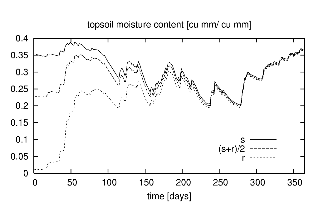
Figure: Simulation of soil moisture in upper soil layer for a soil that is initially at saturation (s), at residual moisture content (r) and in between ([s+r]/2)
What is clear from the Figure is that the initial amount of moisture in the soil only has a marked effect on the start of each simulation; after a few months the three curves converge. In other words, the “memory” of the upper soil layer only goes back a few months (or, more precisely, for time lags of more than about 8 months the autocorrelation in time is negligible).
In theory, this behaviour provides a convenient and simple way to initialise a model such as LISFLOOD. Suppose we want to do a simulation of the year 1995. We obviously don’t know the state of the soil at the beginning of that year. However, we can get around this by starting the simulation a bit earlier than 1995, say one year. In that case we use the year 1994 as a warm-up period, assuming that by the start of 1995 the influence of the initial conditions (i.e. 1-1-1994) is negligible. The very same technique can be applied to initialise LISFLOOD’s other state variables, such as the amounts of water in the lower soil layer, the upper groundwater zone, the lower groundwater zone, and in the channel.
The theory of initialisation
When setting up a model run that includes a warm-up period, most of the internal state variables can be simply set to 0 at the start of the run. This applies to the initial amount of water on the soil surface (WaterDepthInitValue), snow cover (SnowCoverInitValue), frost index (FrostIndexInitValue), interception storage (CumIntInitValue), and storage in the upper groundwater zone (UZInitValue). The initial value of the ‘days since last rainfall event’ (DSLRInitValue) is typically set to 1.
For the remaining state variables, initialisation is somewhat less straightforward. The amount of water in the channel (defined by TotalCrossSectionAreaInitValue) is highly spatially variable (and limited by the channel geometry). The amount of water that can be stored in the upper and lower soil layers (ThetaInit1Value, ThetaInit2Value) is limited by the soil’s porosity. The lower groundwater zone poses special problems because of its overall slow response (discussed in a separate section below). Because of this, LISFLOOD provides the possibility to initialise these variables internally, and these special initialisation methods can be activated by setting the initial values of each of these variables to a special ‘bogus’ value of -9999. The following Table summarises these special initialisation methods:
Table: LISFLOOD special initialisation methods$^1$
| Variable | Description | Initialisation method |
|---|---|---|
| ThetaInit1Value / ThetaForestInit2Value |
initial soil moisture content upper soil layer (V/V) |
set to soil moisture content at field capacity |
| ThetaInit2Value / ThetaForestInit2Value |
initial soil moisture content lower soil layer (V/V) |
set to soil moisture content at field capacity |
| LZInitValue / LZForestInitValue |
initial water in lower groundwater zone (mm) |
set to steady-state storage |
| TotalCrossSectionArea InitValue |
initial cross-sectional area of water in channels |
set to half of bankfull depth |
| PrevDischarge | Initial discharge | set to half of bankfull depth |
$^1$ These special initialisation methods are activated by setting the value of each respective variable to a ‘bogus’ value of “-9999”*
Note that the “-9999” ‘bogus’ value can only be used with the variables in the Table above; the use of the ‘bogus’ value for all the other variables will produce nonsense results! For this reason, the initialisation of the lower groundwater zone is necessary.
WARNING! In areas with arid climate and very thick (~10^2) soils, the use of initial soil water content equal to field capacity creates nonrealistic large discharge values in the channels.
To avoid nonrealistic results in such specific contexts, it is recommended to use the end states of the initialization run to initialize the soil and upper groundwater zone storages of the cold run.
The following end states can be used for the initialization of the run: upper groundwater zone water content; water content of soil layers 1,2,3 for the all the land use categories (other, forest, irrigation).
In summary, the initialization of the lower groundwater zone is always necessary (see paragraph below); the use of the end states to initialize the upper groundwater zone water content and the water content of soil layers 1,2,3 is optional.
This optional, extensive initialization has been implemented in OS-LISFLOOD v4.0.0. The interested users can then use the provided templates as an example to prepare their own initialization run and run with cold start. Please note that the content of this paragraph does not apply to the runs with warm start!
Initialisation of the lower groundwater zone Even though the use of a sufficiently long warm-up period usually results in a correct initialisation, a complicating factor is that the time needed to initialise any storage component of the model is dependent on the average residence time of the water in it. For example, the moisture content of the upper soil layer tends to respond almost instantly to LISFLOOD’s meteorological forcing variables (precipitation, evapo(transpi)ration). As a result, relatively short warm-up periods are sufficient to initialise this storage component. At the other extreme, the response of the lower groundwater zone is generally very slow (especially for large values of $T_{lz}$). Consequently, to avoid unrealistic trends in the simulations, very long warm-up periods may be needed. The Figure below shows a typical example for an 8-year simulation, in which a decreasing trend in the lower groundwater zone is visible throughout the whole simulation period. Because the amount of water in the lower zone is directly proportional to the baseflow in the channel, this will obviously lead to an unrealistic long-term simulation of baseflow. Assuming the long-term climatic input is more or less constant, the baseflow (and thus the storage in the lower zone) should be free of any long-term trends (although some seasonal variation is normal). In order to avoid the need for excessive warm-up periods, LISFLOOD is capable of calculating a ‘steady-state’ storage amount for the lower groundwater zone. This steady state storage is very effective for reducing the lower zone’s warm-up time. The concept of steady state is explained in the LISFLOOD model description, here we will show how it can be used to speed up the initialisation of a LISFLOOD run.
Steady-state storage in practice An actual LISFLOOD simulation differs from the theoretical steady state in 2 ways. First, in any real simulation the inflow into the lower zone is not constant, but varies in time. This is not really a problem, since $LZ_{ss}$ can be computed from the average recharge. However, this is something we do not know until the end of the simulation! Also, the inflow into the lower zone is controlled by the availability of water in the upper zone, which, in turn, depends on the supply of water from the soil. Hence, it is influenced by any calibration parameters that control behaviour of soil- and subsoil (e.g. $T_{uz}$, $GW_{perc}$, $b$, and so on). This means that -when calibrating the model- the average recharge will be different for every parameter set. Note, however, that it will always be smaller than the value of $GW_{perc}$, which is used as an upper limit in the model. As an alternative to using the internal initialization (and hence the bogus values), LZavin and AvgDis (LZInitValue and PrevDischarge) can be computed using an initialization run (or pre-run). The pre-run procedure must include a sufficiently long warm-up period to allow the computation of reliable values of LZavin and AvgDis. The set-up of the initialization run is explained below: the protocol differs slightly depending on the settings of the option split routing.
What you need to do:
Option 1: If using Kinematic routing only (no split routing):
1) Set initial state of all state variables to either 0,1 or -9999 (i.e. cold start with default values or internally initialized values) in Settings.XML file
2) Activate the “InitLisfloodwithoutsplit” and the “InitLisflood” options in
       <setoption choice="1" name="InitLisflood"/>
       <setoption choice="1" name="InitLisfloodwithoutsplit"/>
3) Activate reporting maps (in NetCDF format) in
    <setoption choice="1" name="repEndMaps"/>
    <setoption choice="1"  name="writeNetcdf"/>
4) Set split routing option to not active in
<setoption choice="0" name="SplitRouting"/>
5) Set the name of the reporting map for average percolation rate from upper to lower groundwater zone in
<textvar name="LZAvInflowMap" value="$(PathOut)/lzavin">
6) Run the model for a longer period (if possible more than 3 years, best for the whole modelling period)
7) Go back to the LISFLOOD settings file, and set the InitLisfloodwithoutsplit to inactive, leaving all other switches as before:
    <setoption choice="0" name="InitLisfloodwithoutsplit"/>
    <setoption choice="0" name="InitLisflood"/>
If using Split routing:
1) Set initial state of all state variables to either 0,1 or -9999 (i.e. cold start with default values or internally initialized values) in Settings.XML file
2) Activate the “InitLisflood” option in
    <setoption choice="0" name="InitLisfloodwithoutsplit"/>
    <setoption choice="1" name="InitLisflood"/>
3) Activate reporting maps (in NetCDF format) in
    <setoption choice="1" name="repEndMaps"/>
    <setoption choice="1"  name="writeNetcdf"/>
4) Set split routing option to active in
<setoption choice="1" name="SplitRouting"/>
5) Set the name of the reporting map for average percolation rate from upper to lower groundwater zone in
<textvar name="LZAvInflowMap" value="$(PathOut)/lzavin">
6) Set the name of the reporting map for average discharge map in
<textvar name="AvgDis" value="$(PathOut)/avgdis">
7) Run the model for a longer period (if possible more than 3 years, best for the whole modelling period)
8) Go back to the LISFLOOD settings file, and set the InitLisflood inactive, leaving all other switches as before:
    <setoption choice="0" name="InitLisfloodwithoutsplit"/>
    <setoption choice="0" name="InitLisflood"/>
What to do after the initialization run - Proceed with a LISFLOOD run
i) Checking the lower zone initialisation
The presence of any initialisation problems of the lower zone can be checked by adding the following line to the ‘lfoptions’ element of the settings file:
<setoption name=" repStateUpsGauges" choice="1"></setoption>
This tells the model to write the values of all state variables (averages, upstream of contributing area to each gauge) to time series files. The default name of the lower zone time series is ‘lzUps.tss’.
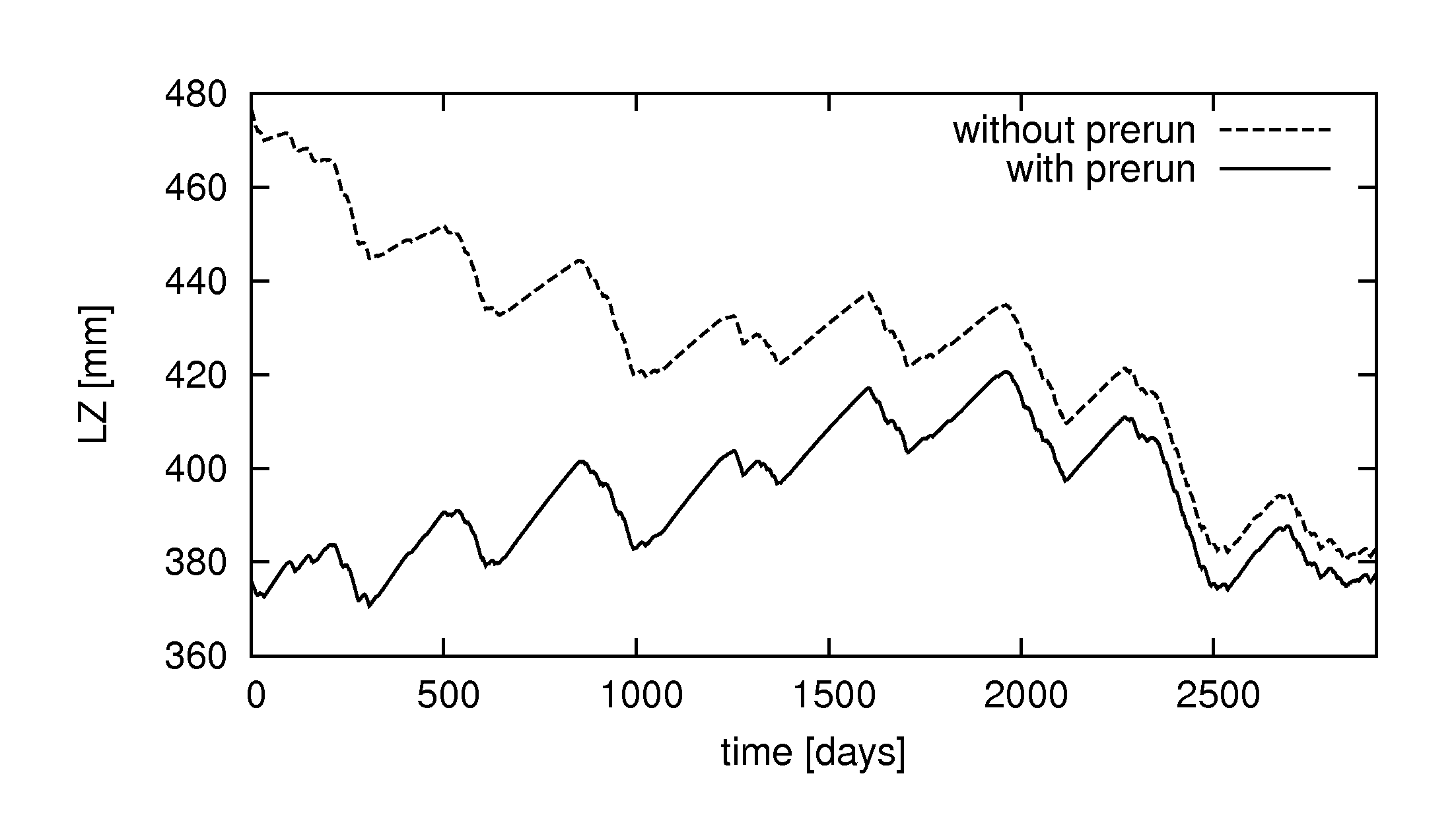
Figure: Initialisation of lower groundwater zone with and without using a pre-run. Note the strong decreasing trend in the simulation without pre-run.
ii) At the end of the initialization run one file (initialization without split routing) or two files (initialization with split routing) will be created in NetCDF format. Copy those files (found in folder “out”, see the setting $(PathOut) above) into the folder “init” ($(PathInit))
lzavin.nc
avgdis.nc
Only the file lzavin.nc is required to run the Lisflood model without split routing.
**************************************************************
INITIAL CONDITIONS FOR THE WATER BALANCE MODEL
(can be either maps or single values)
**************************************************************
</comment>

<textvar name="LZAvInflowMap" value="$(PathInit)/lzavin">
<comment>
$(PathInit)/lzavin.map
Reported map of average percolation rate from upper to
lower groundwater zone (reported for end of simulation)
</comment>
</textvar>

<textvar name="AvgDis" value="$(PathInit)/avgdis">
<comment>
$(PathInit)/avgdis.map
CHANNEL split routing in two lines
Average discharge map [m3/s]
</comment>
</textvar>
iii) launch LISFLOOD
To run the model, start up a command prompt (Windows) or a console window (Linux) and type ‘lisflood’ followed by the name of the settings file, e.g.:
lisflood settings.xml
Important note:
- Calibration parameters obtained with no split routing should never be used to run simulations with split routing and vice versa.
- Using option InitLisfloodwithoutsplit=1 will result in an AvgDis file with zero values everywhere.
- In case of doubts, check content of AvgDis file: if it’s all zero, then split routing must be off. Note that an AvgDis file containing all zero values will automatically set LISFLOOD to no split routing, even if SplitRouting=1.