Step 3: Input files (maps and tables)
In the current version of LISFLOOD, all the model inputs are provided as either maps (grid files in PCRaster format or NetCDF format) or text files (.txt extension). This chapter provides an overview of the data set that is required to run the model.
INPUT MAPS
LISFLOOD requires that all maps must have identical location attributes (number of rows, columns, cellsize, upper x and y coordinates).
The input maps can be classified according to two main cathegories:
- meteorological forcings. These maps provide time series of values for each pixel of the computational domain. More specifically, the meteorological forcings provide the values of precipitation, temperature, reference values of evaporation from water surfaces, reference values of evaporation from open water bodies, reference values of evapotranspiration for each pixel of the modelled area. For each meteorological forcing, one map is required for each computational time step.
- static maps. These maps provide information of morphological, physical, soil, and land use properties for each pixel of the computational domain.
Meteorological forcings
The meteorological forcing variables are defined in map stacks. A map stack is simply a series of maps, where each map represents the value of a variable at an individual time step.
It is recommented to use the netcdf format.
The users that prefer to prepare the meteorological forcings maps in pcraster format, must name the files according to the following rules: the name of each map is made up of a total of 11 characters: 8 characters, a dot and a 3-character suffix. Each map name starts with a prefix, and ends with the time step number. All character positions in between are filled with zeros (“0”).
Generally used prefixes for the meteorological forcings maps are:
- tp : total precipitation; units: mm/day.
- ta : average daily temperature at 2m; units: degrees Celsius or Kelvin (the units must be specified in the settings file)
- EW0 : reference value of evaporation from open water bodies; units: mm/day; these data can be prepared using LISVAP.
- ES0 : reference value of evaporation from bare soil; units: mm/day; these data can be prepared using LISVAP.
- ET0 : reference value of evapotranspiration; units: mm/day; these data can be prepared using LISVAP.
Static maps
The section Static Maps provides detailed guidelines for the preparation of the static maps data set. The following paragraph provides an overview of the different piecies of information provided by the static maps.
- general maps: area mask; landuse mask; grid-cell length; grid-cell area.
- topography: local drain direction; gradient; standard deviation of elevation; upstream area.
- land use maps: fraction of forest; fraction of irrigated crops; fraction of rice crops; fraction of inland water; fraction of sealed surfaces; fraction of other land uses.
- land use depending:crop coefficient; crop group number; Manning/s’s surface roughness; soil depth.
- soil hydraulic properties: saturated hydraulic conductivity; soil water content at saturation; residual soil water content; parameters alpha and lambda of Van Genuchten’s equations.
- channel geometry: channels mask; channels side slope; channels length; channels gradient; Manning’s rougheness coefficient of the channels; channels bottom width; floodplain width; bankfull channels depth.
- leaf area index: evolution of vegetation over time (leaf area index) for land covers forest, irrigated areas, others.
- reservoirs and lakes: lake mask; lakes ID points; reservoirs ID points. These maps are required only upon activation of the lakes module and/or of the reservoirs module.
- rice calendar: rice calendar for planting and harvesting seasons. These maps are required only when activating the rice irrigation module
- inflow points: locations and IDs of the points in which LISFLOOD adds an inflow hydrograph, as explained here
- water demand maps: domestic, energetic, livestock, industrial water use. These maps represent the time series of spatially distributed values of water demand for domestic, energetic, livestock, and industrial water use. These maps are required only when activating the water use module
- outlet points: locations and IDs of the points for which LISFLOOD provides the time series of discharge values.
Role of “mask” and “channels” maps
The mask map (i.e. “area.map”) defines the model domain. In order to avoid unexpected results, it is vital that all maps that are related to topography, land use and soil are defined (i.e. don’t contain a missing value) for each pixel that is “true” (has a Boolean 1 value) on the mask map. The same applies for all meteorological input and the Leaf Area Index maps. Similarly, all pixels that are “true” on the channels map must have some valid (non-missing) value on each of the channel parameter maps. Undefined pixels can lead to unexpected behaviour of the model, output that is full of missing values, loss of mass balance and possibly even model crashes. Some maps needs to have values in a defined range e.g. the gradient map has to be greater than 0.
Geometrical properties of the computational grid cell
LISFLOOD needs to know the size properties of each grid cell (length, area) in order to calculate water volumes from meteorological forcing variables that are all defined as water depths. By default, LISFLOOD obtains this information from the location attributes of the input maps. This will only work if all maps are in an “equal area” (equiareal) projection, and the map co-ordinates (and cell size) are defined in meters. For datasets that use, for example, a latitude-longitude system, neither of these conditions is met. In such cases you can still run LISFLOOD if you provide two additional maps that contain the length and area of each grid cell
Table: Optional maps that define grid size
| Map | Default name | Description |
|---|---|---|
| PixelLengthUser | pixleng.map/nc | Map with pixel length Unit: $[m]$, Range *of values: map > 0 |
| PixelAreaUser | pixarea.map/nc | Map with pixel area Unit: $[m^2]$, Range of values: map > 0 |
Both maps should be stored in the same directory where all other input maps are. The values on both maps may vary in space. A limitation is that a pixel is always represented as a square, so length and width are considered equal (no rectangles). In order to tell LISFLOOD to use the maps a, you need to activate the special option “gridSboveizeUserDefined”, which involves adding the following line to the LISFLOOD settings file:
<setoption choice="1" name="gridSizeUserDefined" \>
LISFLOOD settings files and the use of options are explained in detail in a dedicated chapter and annex of this document.
Leaf area index maps
Because Leaf area index maps follow a yearly circle, only a map stack of one year is necessary which is then used again and again for the following years (this approach can be used for all input maps following a yearly circle e.g. water use). LAI is therefore defined as sparse map stack with a map every 10 days or a month. After one year the first map is taken again for simulation.
Important technical note for the generation of the water regions map
Water demand and water abstraction are spatially distributed within each water region. As detailed here, the water resources (surface water bodies and groundwater) are shared inside the water region in order to meet the cumulative requirements of the water region area. For this reason, it is strongly recommended to include the entire water region(s) in the modelled area. If a portion of the water region is not included in the modelled area, then LISFLOOD cannot adequately compute the water demand and abstraction. In other words, LISFLOOD will not be able to account for sources of water outside of the computational domain (it is important to notice that LISFLOOD will not crush but the results will be affected by this discrepancy). The inclusion of the complete water region in the computational domain becomes compulsory under the specific circumstances of model calibration. Calibrated parameters are optimised for a specific model set up. It is often required to calibrate the parameters of several subcatchments inside a basin. Each calibration subcatchment must include a finite number of water regions (each water region can belong to only one subctatchment). If this condition is met, the calibrated parameters can be correctly optimised. Conversely, when a water region belongs to one or more calibration sub-catchments, the water resources are allocated and abstracted in different quantities when modelling the calibration subcatchment only or the entire basin. Similarly, the option groundwater smooth leads to different geometries of the cone of depression due to groundwater abstraction when modelling the subcatchment only or the entire basin. These two scenarios impede the correct calibration of the model parameters and must be avoided. The user is advised to switch off the groundwater smooth option and to ensure the consistency between water regions and calibration cacthments. The utility waterregions can be used to 1) verify the consistency between calibration catchments and water regions or 2) create a water region map which is consistent with a set of calibration points.
INPUT TABLES
The geographical location of lakes and reservoirs is identified by the two maps described here. These maps provide the location of lakes and reservoirs. Each lake and each reservoir is identified by its ID (a in integer number). LISFLOOD requires additional information for the adequate modelling of lakes and reservoirs. These additional pieces of information are supplied to the numerical code by using tables in .txt format. Each table has 2 colums: the first column is the ID of the lake or of the reservoir, the second column is the quantity required by LISFLOOD. The table below provides the list of the pieces of information which are required for the adequate modelling of lakes and reservoirs.
Table: LISFLOOD input tables
| Table | Default name | Description |
|---|---|---|
| Lake area | Lakearea.txt | Lake syrface area in m2 |
| Lake alpha parameter | lakea.txt | Lake parameter alpha: a detailed descrpition can be found here |
| Lake average inflow | lakeaverageinflow.txt | Average inflow to the lake: a detailed descrpition can be found here |
| Reservoir storage | rstor.txt | Volume in m3, total reservoirs storage capacity |
| Reservoir minimum outflow | rminq.txt | Discharge in m3/s. |
| Reservoir normal outflow | rnormq.txt | Discharge in m3/s. |
| Reservoir non damaging outflow | rndq.txt | Discharge in m3/s. |
| Reservoir conservative storage value | rclimq.txt | Fraction, typical value: 0.07 |
| Reservoir storage limit in normal flow condition | rnlim.txt | Fraction, typical values: 0.65-0.67 |
| Reservoir storage limit during floods | rflim.txt | Fraction, typical value: 0.97 |
Organisation of input data
It is up to the user how the input data are organised. However, it is advised to keep the base maps, meteorological maps and tables separated (i.e. store them in separate directories). For practical reasons the following input structure is suggested:
-
all base maps are in one directory (e.g. ‘maps’)
-
fraction maps in a subfolder (e.g. ‘fraction’)
-
soil hydraulic properties in a subfolder (e.g.’soilhyd’)
-
land cover depending maps in a subfolder (e.g.’table2map’)
-
-
all tables are in one directory (e.g. ‘tables’)
-
all meteorological input maps are in one directory (e.g. ‘meteo’)
-
a folder Leaf Area Index (e.g. ‘lai’)
-
all Leaf Area Index for forest in a subfolder (e.g.’forest’)
-
all Leaf Area Index for other in a subfolder (e.g.’other’)
-
-
all output goes to one directory (e.g. ‘out’)
The following Figure illustrates this:
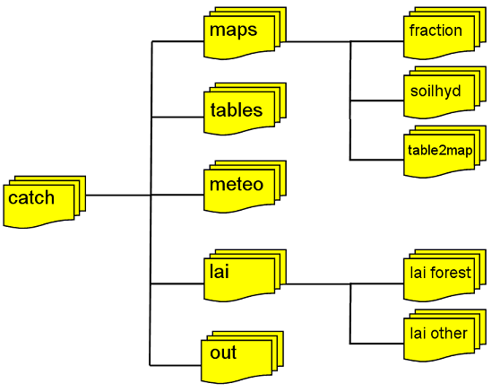
Figure: Suggested file structure for LISFLOOD