## Groundwater storage and sub-surface runoff
Groundwater storage and transport are modelled using two parallel linear reservoirs, similar to the approach used in the HBV-96 model (Lindström et al., 1997). The upper zone represents a quick sub-surface runoff component, which includes fast groundwater and subsurface flow through macro-pores in the soil. The lower zone represents the slow groundwater component that generates the base flow.
Outflow from the [upper groundwater zone](../2_13_stdLISFLOOD_groundwater/index.md#upper-groundwater-zone) (quick sub-surface runoff) and from the [lower groundwater zone](../2_13_stdLISFLOOD_groundwater/index.md#lower-groundwater-zone) (base flow) is added up to generate the [sub-surface runoff](../2_13_stdLISFLOOD_groundwater/index.md#sub-surface-runoff).
### Upper groundwater zone
The **outflow from the upper zone to the channel**, $Q_{uz} [mm]$ equals:
$$
Q_{uz} = \frac{1}{T_{uz}} \cdot UZ \cdot \Delta t
$$
where $T_{uz}$ is the reservoir constant for the upper groundwater layer $[days]$ and $UZ$ is the amount of water that is stored in the upper zone $[mm]$.
Smaller values of $T_{uz}$ lead to a quick response and hence a relatively short residence time of the water in the upper groundwater zone.
The amount of water stored in the upper zone $UZ$ is then updated as follows:
$$
UZ = D_{2,gw} + D_{pref,gw} - D_{uz,lz} - Q_{uz}
$$
where $D_{2,gw}$ is the flux from the lower soil layer to groundwater for each time step; $D_{pref,gw}$ is the amount of preferential flow per each time step; $D_{uz,lz}$ is the amount of **water that percolates from the upper to the lower zone** for each time step, all in $[mm]$.
$D_{2,gw}$ is the weighted sum of the vertical downward fluxes from the three land cover fractions.
In areas with drained irrigation ($DrainedFraction$), the flux from the lower soil layer to groundwater $D_{2,gw}$ is directly delivered to the river channel, consequently, the computation of $UZ$ is modifies as follows:
$$
UZ = (1 - DrainedFraction) \cdot D_{2,gw} + D_{pref,gw} - D_{uz,lz} - Q_{uz}
$$
In areas with flooded irrigation (e.g. rice crops), an additional amount of water is added to $UZ$ during the percolation and draining phases of the agricultural cycle (*RicePercolationWater* and *RiceDrainageWater* are described in a [dedicated chapter](../3_06_optLISFLOOD_paddy-rice/index.md).
The **water percolates from the upper to the lower zone** ($D_{uz,lz}$) is the inflow to the lower groundwater zone. As indicated above, this amount of water is provided by the upper groundwater zone. $D_{uz,lz}$ is a fixed amount per computational time step and it is defined as follows:
$$
D_{uz,lz} = min (GW_{perc} \cdot \Delta t ,UZ)
$$
Here, $GW_{perc} [\frac{mm}{day}]$ is the maximum percolation rate from the upper to the lower groundwater zone.
### Lower groundwater zone
The **outflow from the lower zone to the channel** is then computed by:
$$
Q_{lz} = \frac{1}{T_{lz}} \cdot LZ \cdot \Delta t
$$
Here, $T_{lz}$ is the reservoir constant for the lower groundwater layer ($[days]$), and $LZ$ is the amount of water that is stored in the lower zone ($[mm]$).
Smaller values of $T_{lz}$ lead to a quick response and hence a relatively short residence time of the water in the lower groundwater zone.
$LZ$ is then updated as follows:
$$
LZ = D_{uz,lz} - Q_{lz} - TotalAbstractionFromGroundWater - GW_{loss} \cdot \Delta t
$$
where $D_{uz,lz}$ is the percolation from the upper groundwater zone ($[mm]$); $TotalAbstractionFromGroundWater$ is the total amount of [**water abstracted from groundwater**](../3_07_optLISFLOOD_water-use/index.md) to comply with domestic,industrial, irrigation, and livestock demand; $GW_{loss}$ is the maximum percolation from the lower groundwater zone ($[\frac{mm}{day}]$).
The amount of water defined by $GW_{loss}$ never rejoins the river channel and it's lost beyond the catchment boundaries or to deep groundwater systems. $GW_{loss}$ is set to zero in catchments were no information is available. The larger the value of $GW_{loss}$, the larger the amount of water that leaves the system.
LISFLOOD hence abstracts groundwater from the Lower Zone (LZ). Groundwater depletion can thus be examined by monitoring the LZ levels between the start and the end of a simulation. Given the intra- and inter-annual fluctuations of LZ, it is advisable to monitor more on decadal periods.
If $LZ$ (lower groundwater amount) decreases below a groundwater hold value ($LZ_{Threshold}$), the baseflow Q_{lz} from the lower groundwater zone to the nearby rivers is zero. When sufficient recharge is added again to raise the $LZ$ levels above the threshold, baseflow will start again. This mimicks the behaviour of some river basins in very dry episodes, where aquifers temporarily lose their connection to major rivers and baseflow is reduced. $LZ_{Threshold}$ values are likely different for various (sub)river basins.
The values of $T_{uz}$ $[days]$, $T_{lz}$ $[days]$, $GW_{perc}$ $[\frac{mm}{day}]$, $GW_{loss}$ $[\frac{mm}{day}]$, and $LZ_{Threshold}$ $[mm]$ are obtained by calibration. To avoid spurious results, when $GW_{perc}$ < $GW_{loss}$, $GW_{perc}$ is set equal to $GW_{loss}$.
In the current model implementation, no limit is imposed to water abstraction from groundwater and LZ can become negative: more details are provided in the chapter [Water use](../3_07_optLISFLOOD_water-use/index.md).
Note seepage from soil to upper groundwater zone and percolation from upper to lower groundwater zone are computed only for the permeable fraction of each pixel: groundwater storage in the direct runoff fraction equals 0.
#### Lower groundwater zone: steady state storage
$D_{uz,lz}$, $Q_{lz}$, and $GW_{loss}$ then define LZ water content under natural conditions (no water use).
Now, let’s do a simple numerical experiment: assuming that $D_{uz,lz}$ is a constant value and $GW_{loss}$ is zero, we can take some arbitrary initial value for $LZ$ and then simulate the development over LZ over time. The Figure below shows the results of two numerical experiments. In the upper Figure, we start with a very high initial storage (1500 mm). The inflow rate is fairly small (0.2 mm/day), and $T_{lz}$ is relatively small (250). What is interesting here is that, over time, the storage evolves asymptotically towards a constant state. In the lower Figure, we start with a much smaller initial storage (50 mm), but the inflow rate is much higher (1.5 mm/day) and so is $T_{lz}$ (1000 days). Here we see an upward trend, again towards a constant value. However, in this case the constant ‘end’ value is not reached within the simulation period, which is mainly because $T_{lz}$ is set to a value for which the response is very slow.
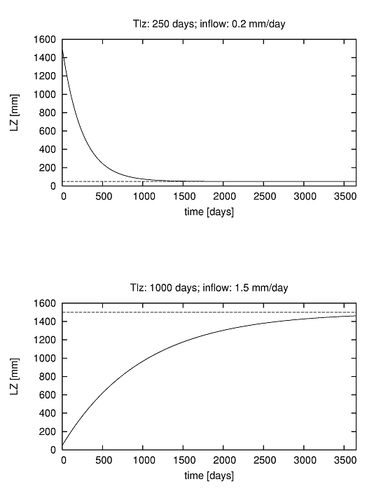 **Figure** Two 10-year simulations of lower zone storage with constant inflow. Upper Figure: high initial storage, storage approaches steady-state storage
(dashed) after about 1500 days. Lower Figure: low initial storage, storage doesn’t reach steady-state within 10 years.
At this point it should be clear that being able to know the ‘end’ storages in the Figure above in advance would be very helpful, because it would eliminate any trend in the water content of the lower groundwater zone. As it happens, this can be done very easily from the model equations. The condition in which *the lower groundwater zone storage is constant over time means that the in- and outflow terms balance each other out*. This condition is known as a **steady state situation**, and the constant ‘end’ storage is in fact the *steady state storage*.
The rate of change of the lower zone’s storage at any moment is given by the continuity equation:
$$
\frac{dLZ}{dt}=I(t)-O(t)
$$
where $I$ is the (time dependent) inflow (i.e. groundwater recharge) and $O$ is the outflow rate. The second governing assumption of the linear storage theory is that:
$$
\frac{LZ}{dt}=O(t)
$$
For a situation where the storage remains constant, we can set:
**Figure** Two 10-year simulations of lower zone storage with constant inflow. Upper Figure: high initial storage, storage approaches steady-state storage
(dashed) after about 1500 days. Lower Figure: low initial storage, storage doesn’t reach steady-state within 10 years.
At this point it should be clear that being able to know the ‘end’ storages in the Figure above in advance would be very helpful, because it would eliminate any trend in the water content of the lower groundwater zone. As it happens, this can be done very easily from the model equations. The condition in which *the lower groundwater zone storage is constant over time means that the in- and outflow terms balance each other out*. This condition is known as a **steady state situation**, and the constant ‘end’ storage is in fact the *steady state storage*.
The rate of change of the lower zone’s storage at any moment is given by the continuity equation:
$$
\frac{dLZ}{dt}=I(t)-O(t)
$$
where $I$ is the (time dependent) inflow (i.e. groundwater recharge) and $O$ is the outflow rate. The second governing assumption of the linear storage theory is that:
$$
\frac{LZ}{dt}=O(t)
$$
For a situation where the storage remains constant, we can set:
$\frac{dLZ}{dt}=0$ only if $I(t)=O(t)$
This equation can be re-written as:
$I(t) - \frac{1}{T_{lz}} \cdot LZ$
Solving this for LZ gives the steady state storage:
$LZ_{ss} = T_{lz} \cdot I(t)$
Applying these equations to the examples above we obtain the *steady state storage* values shown in the Figure.
|$T_{lz}$ | I(t) | $LZ_{ss}$ |
|--------|-------|---------|
|250 | 0.2 | 50 |
|1000 | 1.5 | 1500 |
LISFLOOD provides the possibility to compute the *steady state storage* values internally, all the instructions are provided in the chapter [Initialisation](https://ec-jrc.github.io/lisflood-code/3_step4_model-initialisation/) of the User Guide.
### Sub-surface runoff
All water that flows out of the upper- and lower- groundwater zone is routed to the nearest downstream channel pixel within one time step.
Recalling that the groundwater equations are valid for the pixel's permeable fraction only,the contribution of each pixel to the channel is given by the sum
$$
Q_{uz} + Q_{lz}
$$
In which Q_{uz} is the sum of the contributions from f_{forest}+f_{other}+f_{irrigated}.
Note that, as with the surface runoff routing, no water is routed *through* the river network at this stage.
[🔝](#top)